2 Simulate the system response to different control inputs using MATLAB. Transfer function models describe the relationship between the inputs and outputs of a system using a ratio of polynomials.
![]()
Transfer Functions In Matlab 3 Methods Of Transfer Function In Matlab
The roots of the denominator polynomial are referred to as the model poles.
. I have a unknown system in simulink model non-linear and I dont know how to get a TF which will describe it in certain interval of input data. Thats how Id approach it. Describe the nature of the systems transient response to a unit-step input and consider issues such as the time to reach a steady-state response and whether or not the transient response exhibits.
Once the transfer functions have been entered you can combine them using arithmetic operations such as addition and multiplication to evaluate the transfer function of a cascaded system. The roots of the numerator polynomial are referred to as the model zeros. Now we will demonstrate how to create the transfer function model derived above within MATLAB.
1 Transform an ordinary differential equation to a transfer function. The model order is equal to the order of the denominator polynomial. Electrical Engineering questions and answers.
Step response using Matlab Example. What are Transfer Function Models. The model order is equal to the order of the denominator polynomial.
Definition of Transfer Function Models. For the series connection of blocks The MATLAB command is SYS G1 G2 or SYS series G1G2 where SYS Y sR s. In linear systems transfer functions depend only on the frequency of the input signal.
Numerically evaluate and plot the impulse step and forced responses of a system. The model order is equal to the order of the denominator polynomial. 720 Figure P720 shows a system defined by a transfer function.
The roots of the denominator polynomial are referred to as the model poles. We have that. With respect to characterizing your system in transfer function form it would likely be best to begin with a state-space representation then use the ss2tf function that is actually part of base MATLAB then the minreal function to guarantee stability.
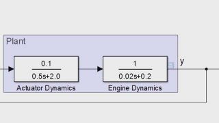
G overall s G 1 s G 2 s The overall transfer function for a system composed of elements in series is the product of the transfer functions of the individual series elements. C Plot the system with MATLAB and give three 3 different scenarios of inputs step ramp sinusoidal and elaborate the plot using the determined and undetermined time. Transfer function models describe the relationship between the inputs and outputs of a system using a ratio of polynomials.
I tried tfestdatanumber_of_polesnumber_of_zeroes Also I tried ident and then import input and output into ident GUI and then. The model order is equal to the order of the denominator polynomial. K is the gain of the factored form.
Parameter Identification of Transfer Functions Using MATLAB u. Mathematical models that describe the system can be given as a result. Bode diagrams are useful in frequency response analysis.
For the transfer function G s Gs 3s2 2s3 4s2 5s1 G s 3 s 2 2 s 3 4 s 2 5 s 1. Derive transfer functions by hand. We can describe a linear system dynamics using differential equations or using transfer functions.
Copy to Clipboard. Transfer functions are a frequency-domain representation of linear time-invariant systems. Give any assumptions needed and its numerical example.
Derive transfer functions using symbolic math. Create the factored transfer function G s 5 s s 1 i s 1 i s 2. An interactive lesson that teaches how to derive transfer functions and compute time responses analytically and in MATLAB.
It is an extension of linear frequency response analysis. By using SIT to obtain transfer function the procedure is faster and simpler than using conventional methods. Transfer function models describe the relationship between the inputs and outputs of a system using a ratio of polynomials.
From the Transfer Function For a transfer function. Obtain a plot of the step response by adding a pole at s 0 to G s and using the impulse command to plot the inverse Laplace transform. B Write the mathematical model and the transfer function.
Use MATLAB to determine the characteristic roots of the system. Enter the following commands into the m-file in which you defined the system parameters. A Describe a system that can be designedmodelled as Fig.
The video accompanying this post is given below. Im sorry that im asking such abstract question but im really lost. In nonlinear systems when a specific class of input signal such as a sinusoid is applied to a.
Sys 1ms2bsk sys 1 ----- s2. This procedure is explained in next few steps. Transfer function models describe the relationship between the inputs and outputs of a system using a ratio of polynomials.
Also known as discrete transfer function. Describe the nature of the systems transient response to a unit-step input and consider issues such as the time to reach a steady-state response and whether or not the transient response exhibits oscillations. The roots of the numerator polynomial are referred to as the model zeros.
Use MATLAB to determine the characteristic roots of the system. P -1-1i -11i -2. Describing function analysis is a technique for studying the frequency response of nonlinear systems.
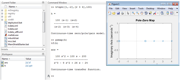
In this post we will learn how to. For instance consider a continuous-time SISO dynamic system represented by the transfer function sys s N sD s where s jw and N s and D s are called the numerator and denominator polynomials respectively. G zpk ZPK.
The roots of the denominator polynomial are referred to as the model polesThe roots of the numerator polynomial are referred to as the model zeros. Pəlst tranzfər faŋkshən control systems The ratio of the z-transform of the output of a system to the z-transform of the input when both input and output are trains of pulses. Analytically derive the step and forced responses of a.
The overall transfer function G s of the system is Y s X s and so. 720 Figure 720 shows a system defined by a transfer function. 𝜔 𝜔 𝜔 Where 𝜔is the frequency response of the system ie we may find the frequency response by setting 𝜔 in the transfer function.
Z and P are the zeros and poles the roots of the numerator and denominator respectively. The disadvantage of this analysis is that an.
Solved 1 We Can Define The Transfer Function Of A System By Chegg Com
Transfer Functions In Matlab 3 Methods Of Transfer Function In Matlab
Transfer Functions In Simulink Part 2 Extracting Transfer Functions Video Matlab


0 Comments